Manifolds

It is a core underlying assumption of both special and general relativity—indeed of much of physics—that spacetime is a continuum: to characterise an event we need four numbers (one temporal, three spatial). In special relativity this continuum is the familiar flat $\mathbb{R}^{4}$, but in general relativity the geometry itself is dynamical—it changes in response to the distribution of matter, energy, and stress throughout the universe.

Because we now allow the geometry to be curved and dynamical, we need a mathematical apparatus to describe and quantify the situation precisely; without it we would be limited to qualitative remarks, whereas in physics we want to make sharp, falsifiable predictions. One approach would be to model curved continua as surfaces embedded in a higher-dimensional ambient space $\mathbb{R}^{m}$. This works, but it raises an uncomfortable question: do these extra dimensions exist? We sidestep the issue entirely by studying curved continua intrinsically, without reference to any ambient space—and this leads us to the theory of manifolds.

Physical intuition

In general relativity, spacetime is a manifold ℳ. Although we may picture ℳ as sitting inside some higher-dimensional ℝ^m, all physically meaningful statements should be intrinsic: they must not depend on the embedding. The intrinsic approach requires more formalism upfront, but it is ultimately more natural and more transferable to other areas of theoretical physics.

Notation and prerequisites

We work in $n$ dimensions throughout. One might ask: why bother with arbitrary $n$ when spacetime is four-dimensional? There are several good reasons. First, it costs almost no extra effort and yields considerable generality for free. Second, we often wish to restrict attention to dynamics on a lower-dimensional hypersurface (a particle constrained to the surface of a sphere, for instance). Third—and more speculatively—there are indications from quantum gravity (the holographic principle, for example) that the effective dimension of spacetime may itself be emergent. Finally, in a quantum theory of gravity one might need to superpose spacetimes of different dimensions, so it is wise not to hard-code $n=4$.

$\mathbb{R}^{n} = \{(x^1,\dots,x^n) \mid x^j \in \mathbb{R}\}$.
For $\boldsymbol{x} = (x^1,\dots,x^n)$, the Euclidean norm is \[\lVert \boldsymbol{x}-\boldsymbol{y} \rVert = \Bigl(\sum_{j=1}^{n}(x^j - y^j)^2\Bigr)^{1/2}.\]
The open ball of radius $r$ about $\boldsymbol{y}$ is \[B_r(\boldsymbol{y}) = \{\boldsymbol{x}\in\mathbb{R}^{n} \mid \lVert \boldsymbol{x}-\boldsymbol{y} \rVert < r\}.\]
A subset $U\subseteq\mathbb{R}^{n}$ is open if for every $\boldsymbol{x}\in U$ there exists $\varepsilon > 0$ such that $B_\varepsilon(\boldsymbol{x})\subset U$.
$C^k$ denotes the set of $k$-times continuously differentiable functions (from $\mathbb{R}^{n}$ to $\mathbb{R}$, or between open subsets thereof): all partial derivatives of order $\le k$ exist and are continuous.
$C^0 = {}$continuous functions, $C^\infty = {}$smooth (infinitely differentiable) functions.

Definition of a manifold

Definition

An n-dimensional, C^∞, real manifold ℳ is a set together with a collection {O_α} of subsets satisfying:

ℳ is a topological space (Hausdorff and second-countable).¹
The subsets {O_α} cover ℳ, i.e. ⋃_αO_α = ℳ. Equivalently: for every p ∈ ℳ there exists at least one α with p ∈ O_α.
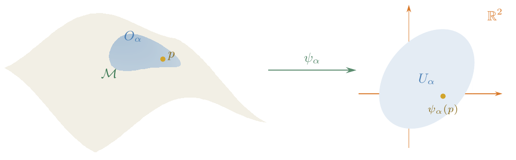
For each α there is a homeomorphism ψ_α : O_α → U_α , U_α ⊂ ℝⁿ (open) ,

A single chart. Chart ψ_α : O_α → U_α ⊂ ℝ² identifies a patch of the manifold with an open set in Euclidean space.

One should think of each pair (O_α,ψ_α) as identifying a piece of the manifold with a piece of Euclidean space. A manifold is thus built up—sewn together—from patches of ℝⁿ.
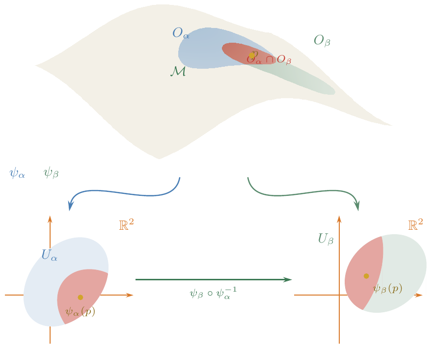
If any two sets O_α and O_β overlap, i.e. O_α ∩ O_β ≠ ⌀, then the transition map ψ_β ∘ ψ_α⁻¹ : ψ_α[O_α∩O_β] → ψ_β[O_α∩O_β] (which is a map between open subsets of ℝⁿ) is C^∞. This condition governs the gluing: wherever two patches overlap, the two coordinate descriptions must be smoothly related.

Charts (Oα, ψα) and (Oβ, ψβ) with overlap Oα ∩ Oβ (red) on the manifold, and the transition map ψβ ∘ ψα<sup>−1</sup> between open subsets of ℝ². — **Two overlapping charts and the transition map.** Charts (O_α, ψ_α) and (O_β, ψ_β) with overlap O_α ∩ O_β (red) on the manifold, and the transition map ψ_β ∘ ψ_α⁻¹ between open subsets of ℝ².

Charts and atlases

The maps $\psi_\alpha$ are called charts (in mathematics) or coordinate systems (in physics).

The definition as stated depends on the choice of cover $\{O_\alpha\}$ and charts $\{\psi_\alpha\}$. Adding a new chart $\psi'$ compatible with the existing ones would formally give a “new” manifold, even though it carries no new information. To eliminate this ambiguity we require the atlas $\{\psi_\alpha\}$ to be maximal: all coordinate systems compatible with conditions (2) and (3) are included.

Physical intuition

Requiring maximality is a bookkeeping device. In practice one specifies a convenient atlas and declares that every compatible chart is implicitly included.

Examples

$\mathbb{R}^{n}$ as a manifold

$\mathbb{R}^{n}$ is the trivial example: it can be covered by a single chart $O_1 = \mathbb{R}^{n}$, $\psi_1 = \id$. As a manifold, $\mathbb{R}^{n}$ has uncountably many compatible covers (any collection of open sets that covers $\mathbb{R}^{n}$, together with the identity or other smooth maps, will do).

Spacetime

Minkowski spacetime is $\mathbb{R}^1\times\mathbb{R}^3 \cong \mathbb{R}^{1,3} \cong \mathbb{R}^{4}$ as a manifold. (The Lorentzian structure—the metric signature—comes later.)

The sphere $S^n$

The $n$-sphere is \[\label{eq:Sn-def} S^n = \bigl\{(x^1,\dots,x^{n+1})\in\mathbb{R}^{n+1} \;\big|\; \textstyle\sum_{j=1}^{n+1}(x^j)^2 = 1\bigr\}.\] $S^n$ cannot be covered by a single chart (it is compact, while any chart image is an open subset of $\mathbb{R}^{n}$). Define the $2(n{+}1)$ open sets \[\label{eq:Sn-open-sets} O_k^+ = \{(x^1,\dots,x^{n+1})\in S^n \mid x^k > 0\}\,, \qquad O_k^- = \{(x^1,\dots,x^{n+1})\in S^n \mid x^k < 0\}\,,\] for $k = 1,\dots,n{+}1$. These cover $S^n$. The corresponding charts are \[\label{eq:Sn-charts} \psi_k^\pm : O_k^\pm \to \mathbb{R}^{n}\,, \qquad \psi_k^\pm(x^1,\dots,x^{n+1}) = (x^1,\dots,x^{k-1},x^{k+1},\dots,x^{n+1})\,,\] i.e. one simply drops the $k$-th coordinate (whose sign is determined by the choice of $O_k^\pm$).

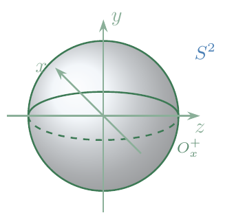
Special case: $S^2$. Consider the charts $\psi_x^+$ (drop $x$, restricted to $x>0$) and $\psi_y^-$ (drop $y$, restricted to $y<0$). On the overlap $\{(y,z)\in\mathbb{R}^{2} \mid y<0,\; y^2+z^2<1\}$, the transition function is \[(\psi_y^-\circ(\psi_x^+)^{-1})(y,z) = \bigl(\sqrt{1-y^2-z^2},\; z\bigr).\]

Stereographic-style axes in ℝ³ and the open upper-x hemisphere Ox<sup>+</sup> = {(x,y,z)∈S² : x > 0}, one of the six coordinate-halving charts of S². — **The 2-sphere S² with chart patch O_x⁺.** Stereographic-style axes in ℝ³ and the open upper-x hemisphere O_x⁺ = {(x,y,z)∈S² : x > 0}, one of the six coordinate-halving charts of S².

Exercise

Find the remaining transition functions for the atlas {ψ_k^±} of Sⁿ and show that they are all C^∞.

Physical intuition

For many basic solutions of Einstein’s field equations the underlying manifold is simply ℝ⁴—only the geometry (the metric) varies. So one might wonder whether the full manifold machinery is really necessary. The answer is yes: as soon as one considers cosmological spacetimes (which may be compact, like S³ × ℝ) or black hole spacetimes (which have non-trivial causal structure and topology), more general manifolds become unavoidable. In quantum gravity one may even wish to sum over manifolds of different topologies, making this generality essential.

New manifolds from old: product manifolds

Suppose $\mathcal{M}$ and $\mathcal{M}'$ are manifolds of dimension $n$ and $n'$, respectively. We can form the product manifold $\mathcal{M}\times\mathcal{M}'$.

Let $\psi_\alpha: O_\alpha\to U_\alpha$ and $\psi'_\beta: O'_\beta\to U'_\beta$ be charts for $\mathcal{M}$ and $\mathcal{M}'$. Define charts for $\mathcal{M}\times\mathcal{M}'$ via \[\psi_{\alpha\beta}: O_\alpha\times O'_\beta \;\to\; U_\alpha\times U'_\beta \;\subset\; \mathbb{R}^{n+n'}\,,\] with \[\label{eq:product-chart} \psi_{\alpha\beta}(p,p') = \bigl(\psi_\alpha(p),\;\psi'_\beta(p')\bigr) \;\in\; \mathbb{R}^{n+n'}\,.\]

Exercise

Verify that ℳ × ℳ′ with the charts {ψ_αβ} satisfies the manifold axioms.

Example

$\mathbb{R}^{n} = \underbrace{\mathbb{R}\times\mathbb{R}\times\cdots\times\mathbb{R}}_{n}$.
The torus: T² = S¹ × S¹.
With just ℝ and Sⁿ and their products, one can construct many of the manifolds relevant to general relativity.

Smooth maps and diffeomorphisms

Let $\mathcal{M}$ and $\mathcal{M}'$ be manifolds with charts $\{\psi_\alpha\}$ and $\{\psi'_\beta\}$.

Definition

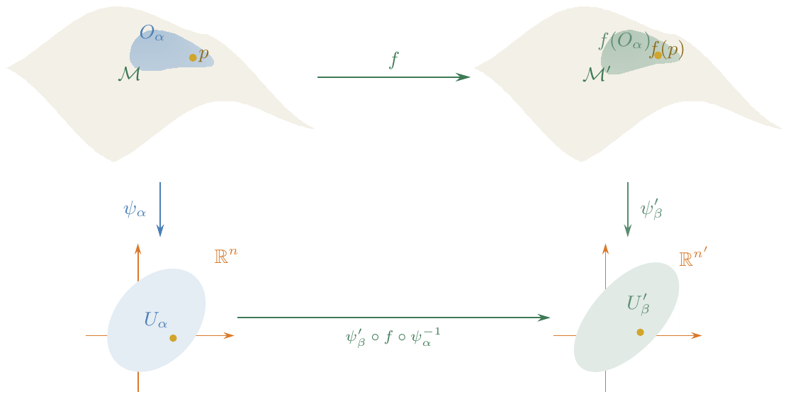
A map f : ℳ → ℳ′ is said to be C^∞ (smooth) if for all α, β the composite ψ′_β ∘ f ∘ ψ_α⁻¹ : U_α → U′_β is C^∞ (as a map between open subsets of Euclidean spaces).

The smooth map f : ℳ → ℳ′ viewed through charts ψα and ψ′β; the composite ψ′β ∘ f ∘ ψα<sup>−1</sup> must be smooth as a map between open subsets of Euclidean space. — **A smooth map between manifolds and its chart representative.** The smooth map f : ℳ → ℳ′ viewed through charts ψ_α and ψ′_β; the composite ψ′_β ∘ f ∘ ψ_α⁻¹ must be smooth as a map between open subsets of Euclidean space.

Definition

A map f : ℳ → ℳ′ is a diffeomorphism if it is C^∞, one-to-one, onto, and its inverse f⁻¹ is also C^∞. If such a map exists, ℳ and ℳ′ are said to be diffeomorphic: they have identical manifold structure.

Vectors on manifolds

Euclidean space $\mathbb{R}^{n}$ (and Minkowski space) carries a natural global vector space structure: $V = \mathbb{R}^{n}$ is simultaneously a manifold and a vector space.

For a general manifold this is no longer true—there is no natural additive structure. This is an instance of a general phenomenon: when one generalises a definition so that it applies to more examples, some of the structure enjoyed by the original example is inevitably lost. Euclidean space is simultaneously a manifold, a vector space, and a group; a generic manifold is none of the latter two.

Example

The 2-sphere S² is a manifold, but it is not a vector space: there is no natural way to “add” two points on S² and obtain another point on S².

We want to preserve as much of this vector-space structure as possible, because without vectors we cannot write down equations of motion for test particles. The key observation is that even though $S^2$ is not globally a vector space, at each point $p$ there is still a natural local vector space—the tangent plane—and this idea generalises to arbitrary manifolds.

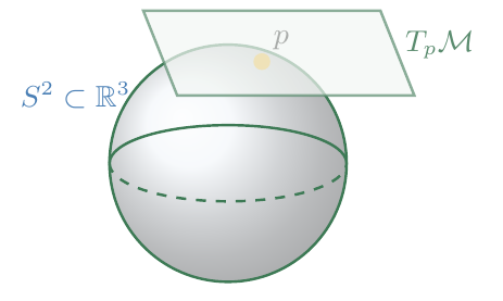
It is, however, still possible to associate a vector space to each point of a manifold. For a manifold $\mathcal{M}$ embedded in $\mathbb{R}^{m}$ (such as $S^2\subset\mathbb{R}^{3}$), one can visualise the tangent plane at a point $p$:

Visualising Tpℳ for S² ⊂ ℝ³. The plane is what one reaches for when the manifold sits inside an ambient space — but this picture relies on the embedding, so the next lecture gives an intrinsic definition. — **Tangent plane to the 2-sphere at a point.** Visualising T_pℳ for S² ⊂ ℝ³. The plane is what one reaches for when the manifold sits inside an ambient space — but this picture relies on the embedding, so the next lecture gives an intrinsic definition.

But we want an intrinsic definition, independent of any embedding.

Key result

The picture above relies on the embedding S² ⊂ ℝ³, which we have declared off-limits. The solution is a pleasant roundabout: one first observes that there is a one-to-one correspondence between tangent vectors and directional derivatives of smooth functions, and then notes that directional derivatives can be defined using only the manifold structure—no embedding required. We therefore define tangent vectors as directional derivatives. This is developed in the next lecture.

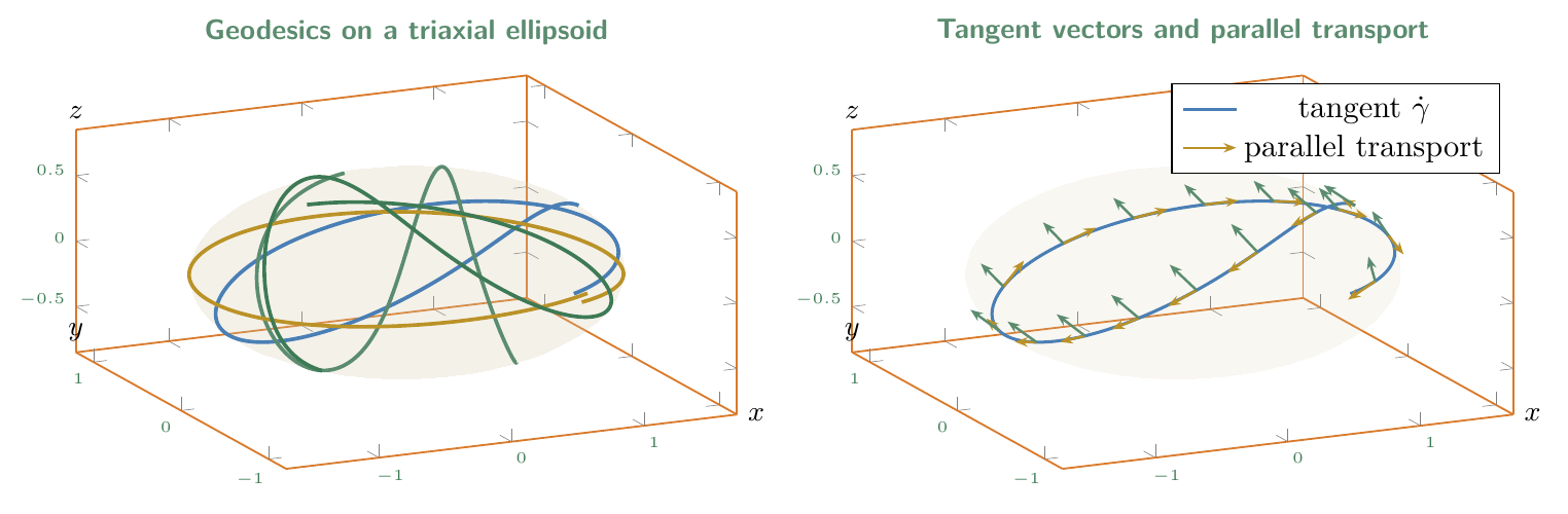
**Geodesics on a triaxial ellipsoid with parallel transport.** Top: geodesics (shortest paths intrinsic to the surface) on a triaxial ellipsoid (a=1.5, b=1.0, c=0.7). Bottom: tangent vectors (gold) and a parallel-transported vector (teal) along a geodesic — parallel transport preserves inner products but the transported vector rotates relative to the tangent direction.

Formal definitions (summary)

We collect the precise versions of the definitions introduced above for reference.

Definition

A locally Euclidean space of dimension d is a Hausdorff topological space ℳ such that every point has a neighbourhood homeomorphic to an open subset of ℝ^d.

Definition

A differentiable structure ℱ of class C^k (1 ≤ k ≤ ∞) on a locally Euclidean space ℳ is a collection of coordinate systems {(O_α,ψ_α) ∣ α ∈ A} such that:

⋃_α ∈ AO_α = ℳ.
ψ_α ∘ ψ_β⁻¹ is C^k for all α, β ∈ A.
The collection ℱ is maximal with respect to (b).

A $d$-dimensional differentiable manifold of class $C^k$ is a pair $(\mathcal{M},\mathcal{F})$ consisting of a second-countable, locally Euclidean space $\mathcal{M}$ together with a differentiable structure $\mathcal{F}$ of class $C^k$. (The $C^k$ condition can be generalised to $C^\infty$, complex analytic, etc.)

Manifolds

Notation and prerequisites

Definition of a manifold

Charts and atlases

Examples

\(\mathbb{R}^{n}\) as a manifold

Spacetime

The sphere \(S^n\)

New manifolds from old: product manifolds

Smooth maps and diffeomorphisms

Vectors on manifolds

Formal definitions (summary)